In many laser optics applications, the laser beam is assumed Gaussian with an irradiance profile that follows an ideal Gaussian distribution. All actual laser beams will have some deviation from ideal Gaussian behavior. The M² factor , also known as the beam quality factor, compares the performance of a real laser beam with that of a diffraction-limited Gaussian beam. Gaussian irradiance profiles are symmetric around the center of the beam and decrease as the distance from the center of the beam perpendicular to the direction of propagation increases (Figure 1).

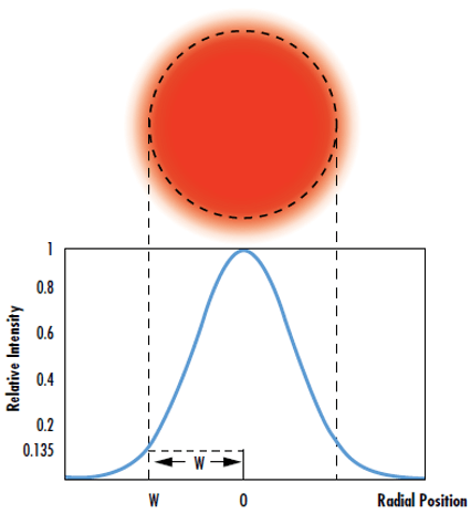
Figure 1: The waist of a Gaussian beam is defined as the location where the irradiance is 1/e² (13.5%) of its maximum value

Equation 1 describes this distribution:

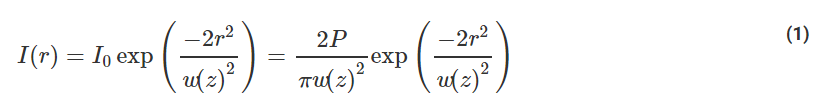
In Equation 1, I₀ is the peak irradiance at the center of the beam,

r is the radial distance away from the axis,

w(z) is the radius of the laser beam where the irradiance is 1/e² (13.5%) of I₀,

z is the distance propagated from the plane where the wavefront is flat,

and P is the total power of the beam.

However, this irradiance profile does not stay constant as the beam propagates through space, hence the dependence of w(z) on z. Due to diffraction, a Gaussian beam will converge and diverge from an area called the beam waist (w₀), which is where the beam diameter reaches a minimum value. The beam converges and diverges equally on both sides of the beam waist by the divergence angle θ (Figure 2). The beam waist and divergence angle are both measured from the axis and their relationship can be seen in Equation 2 and Equation 3:

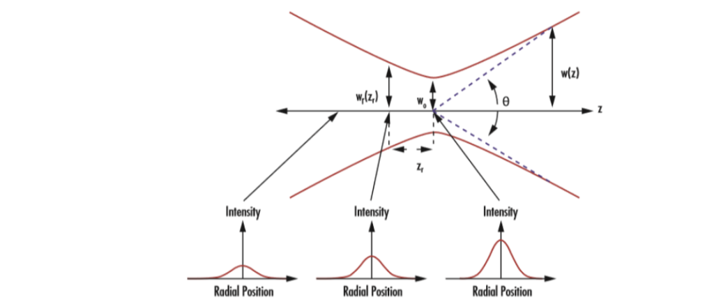
Figure 2: Gaussian beams are defined by their beam waist (w₀), Rayleigh range (z_R), and divergence angle (θ)

Variation of the beam diameter in the beam waist region is defined by:

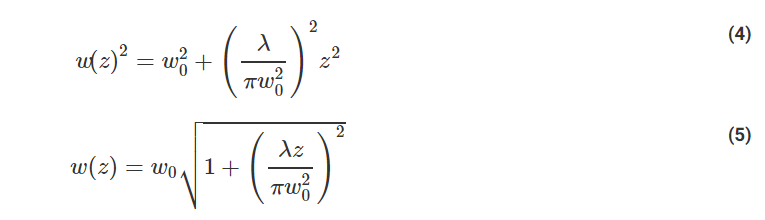
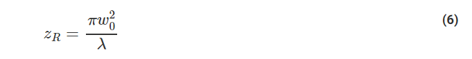
The Rayleigh range of a Gaussian beam is defined as the value of z where the cross-sectional area of the beam is doubled. This occurs when w(z) has increased to √2 w₀. Using Equation 5, the Rayleigh range (z_R) can be expressed as:

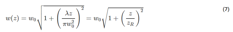
This allows w(z) to also be related to z_R:

The wavefront of the laser is planar at the beam waist and approaches that shape again as the distance from the beam waist region increases. This occurs because the radius of curvature of the wavefront begins to approach infinity. The radius of curvature of the wavefront decreases from infinity at the beam waist to a minimum value at the Rayleigh range, and then returns to infinity when it is far away from the laser (Figure 3); this is true for both sides of the beam waist.

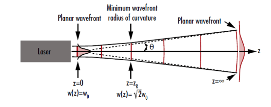
Figure 3: The curvature of the wavefront of a Gaussian beam is near-zero when it is both very close and very far away from the beam waist

Gaussian Beam Manipulation

Many laser optics systems require manipulation of a laser beam as opposed to simply using the “raw” beam. This may be done using optical components such as lenses, mirrors, prisms, etc. Below is a guide to some of the most common manipulations of Gaussian beams.

The Thin Lens Equation for Gaussian Beams

The behavior of an ideal thin lens can be described using the following equation:

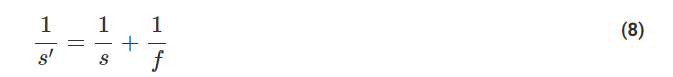
In Equation 8, s’ is the distance from the lens to the image, s is the distance from the lens to the object, and f is the focal length of the lens. If the object and image are at opposite sides of the lens, s is a negative value and s’ is a positive value. This equation ignores the thickness of a real lens and is therefore only a simple approximation of real behavior (Figure 4). The thin lens equation can also be written in a dimensionless form by multiplying both sides of the equation by f:

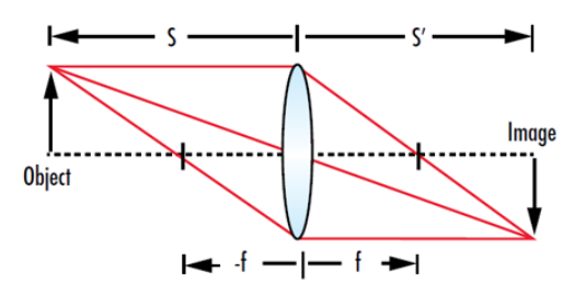
Figure 4: The thin lens equation allows the position of an image (s’) to be determined when the distance from the lens to the object (s) and the focal length of the lens (f) are known

In addition to describing imaging applications, the thin lens equation is applicable to the focusing of a Gaussian beam by treating the waist of the input beam as the object and the waist of the output beam as the image. Gaussian beams remain Gaussian after passing through an ideal lens with no aberrations. In 1983, Sidney Self developed a version of the thin lens equation that took Gaussian propagation into account:

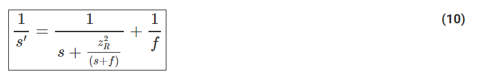
The total distance from the laser to the focused spot is calculated by adding the absolute value of s to s’. Equation 10 can also be written in a dimensionless form by multiplying both sides by f:

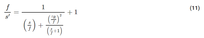
This equation approaches the standard thin lens equation as z_R/f approaches 0, allowing the standard thin lens equation to be used for lenses with a long focal length. Equations 10 and 11 can be used to find the location of the beam waist after being imaged through the lens (Figure 5).

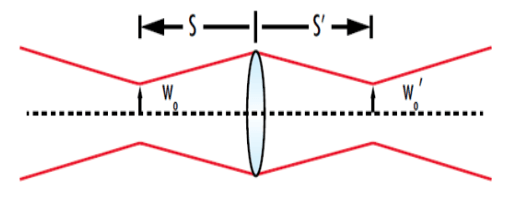
Figure 5: The ”object” when refocusing a Gaussian beam is the input waist and the “image” is the output waist

A plot of the normalized image distance (s’/f) versus the normalized object distance (s/f) shows the possible output waist locations at a given normalized Rayleigh range (z_R/f) (Figure 6). This plot shows that Gaussian beams focused through a lens have a few key differences when compared to conventional thin lens imaging. Gaussian beam imaging has both minimum and maximum possible image distances, while conventional thin lens imaging does not. The maximum image distance of a refocused Gaussian beam occurs at an object distance of -(f + z_R), as opposed to –f. The point on the plot where s/f is equal to -1 and s’/f is equal to 1 indicates that the output waist will be at the back focal point of the lens if the input is at the front focal point of a positive lens.

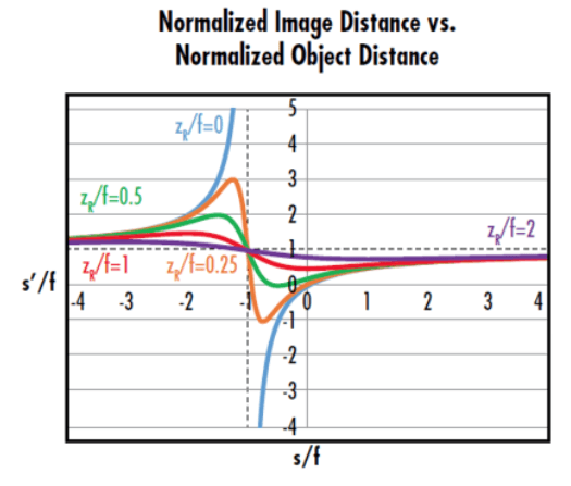
Figure 6: The curve where z_R/f=0 corresponds to the conventional thin lens equation. The curves where z_R/f>0 show that Gaussian imaging has minimum and maximum image distances defined by the Rayleigh range

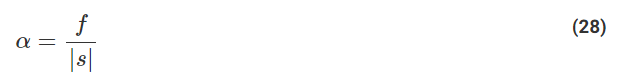
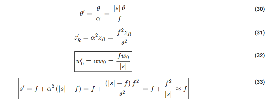
In order to understand the beam waist and Rayleigh range after the beam travels through the lens, it is necessary to know the magnification of the system (α), given by:

Where w₀ is beam waist before the lens and w₀’ is the beam waist after the lens. The thin lens equation for Gaussian beams can then be rewritten to include the Rayleigh range of the beam after the lens (z_R‘):

The above equation will break down if the lens is at the beam waist (s=0). The inverse of the squared magnification constant can be used to relate the beam waist sizes and locations:

Focusing a Gaussian Beam to a Spot

In many applications, such as laser materials processing or surgery, it is highly important to focus a laser beam down to the smallest spot possible to maximize intensity and minimize the heated area. In cases such as these, the goal is to minimize w₀‘ (Figure 7). A modified version of Equation 14 may be used to identify how to minimize the output beam waist:

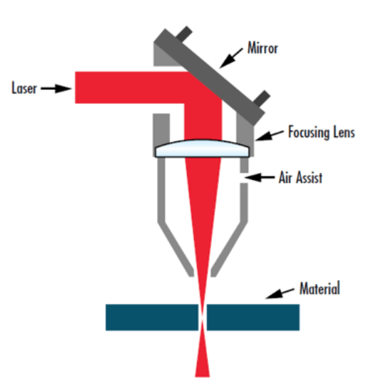
Figure 7: Focusing a laser beam down to the smallest possible size is crucial for a wide range of applications including this laser cutting setup

After multiplying both sides by the denominator from the left side of the equation and then multiplying both sides by (w₀‘)^², Equation 15 becomes:

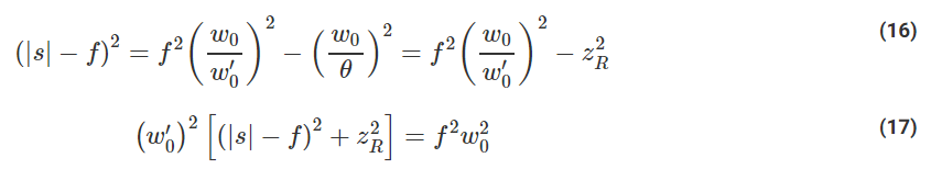
Solving for w₀‘ results in:

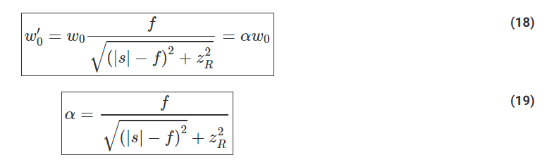
The focused beam waist can be minimized by reducing the focal length of the lens and |s|-f. The terms next to w₀ in Equation 18 are defined as another form of the magnification constant α in order to compare the values of the input beam to the output beam after going through the lens (Figure 8).

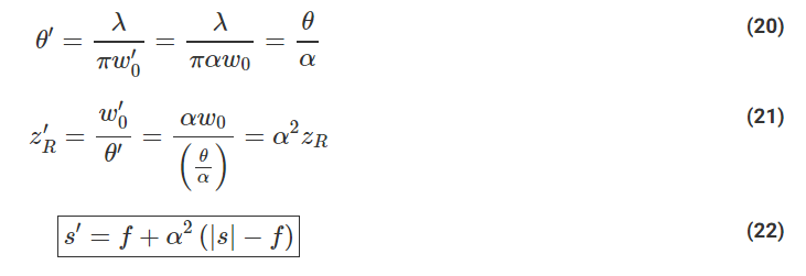
Figure 8: For a magnification of 2, the output beam waist will be twice the input beam waist and the output divergence will be half of the input beam divergence

There are two limiting cases which further simplify the calculations of the output beam waist size and location: when s is much less than z_R or much greater than z_R. When the lens is well within the laser’s Rayleigh range, then s << z_R and (|s|-f)²<〖z_R〗². Equation 19 simplifies to:

This also simplifies the calculations for the output beam’s waist, divergence, Rayleigh range, and waist location:

The other limiting situation where the lens is far outside of the Rayleigh range and s >> z_R, simplifying Equation 19 to:

Which makes the output beam waist diameter:

Similarly to when s << z_R, the calculations for the output beam waist, divergence, Rayleigh range, and beam waist location are also simplified:

When s >> z_R, the distance from the lens to the focused spot equals the focal length of the lens.

Both of these results intuitively make sense because the beam’s wavefront is approximately planar both at and very far away from the beam waist. At these locations, the beam is almost perfectly collimated (Figure 9). According to the standard thin lens equation, a collimated input would have an image distance equal to the focal length of the lens.

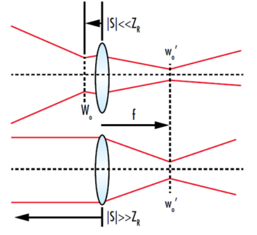
Figure 9: The focused spot of a Gaussian beam after it passes through a lens will be located at the focal point of the lens if the input beam waist is either very close or very far away from the lens. This is because the input beam is approximately collimated at those points

Gaussian Focal Shift

Counterintuitively, the intensity of a focused beam in a target at a fixed distance (L) away from the lens is not maximized when the waist is located at the target. The intensity on the target is actually maximized when the waist occurs at a location before the target (Figure 10). This phenomenon is known as Gaussian focal shift.

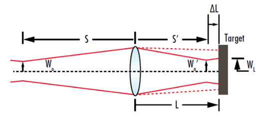
Figure 10: The minimum beam radius at a target occurs when the waist of the focused beam occurs at a specific location before the target, not when focused waist is located at the target

The lengthy derivation is not covered in this text, but the beam radius at the target can be described by the following expression:

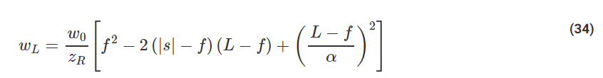
Differentiating Equation 34 with respect to the focal length of the focusing lens (f) and solving for f when ^d⁄_df [w_L (f )]=0 reveals the lens focal length resulting in the minimum beam radius, and therefore highest intensity, at the target.

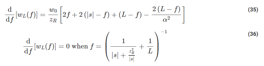
As |s| approaches either zero or infinity, ^d⁄_df [w_L (f )]=0 when f=L. In both of these cases, the input beam is approximately collimated, and it thereby follows that the smallest beam radius would occur at the focal point of the lens.

Collimating a Gaussian Beam

Achieving a truly collimated beam where the divergence is 0 is not possible, but achieving an approximately collimated beam by either minimizing the divergence or maximizing the distance between the point of observation and the nearest beam waist is possible. Since the output divergence is inversely proportional to the magnification constant α, the output divergence reaches a minimum value when |s|= f (Figure 11)

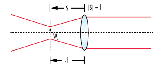
Figure 11: To collimate a Gaussian beam, the distance from the beam waist to the collimating lens should be equal to the lens’ focal length

References

“Gaussian Beam Optics.” CVI Laser Optics, IDEX Optics & Photonics.
O’Shea, Donald C. Elements of Modern Optical Design. Wiley, 1985.
Self, Sidney A. “Focusing of Spherical Gaussian Beams.” Applied Optics, vol. 22, no. 5, Jan. 1983.

How Laser beam is transmitted?